VLOOKUP in Excel: A Complete Guide

When it comes to working with large and complex data sets in Excel, finding and retrieving the information you need can be challenging. You may waste a lot of time and effort scrolling through rows and columns or writing complicated formulas. That's why you need to understand VLOOKUP in Excel.

VLOOKUP is a powerful function that can help you look up and match data from different tables and return the results you want. In this blog, we will teach you everything you need to know about VLOOKUP in Excel, from the basics to the advanced tips and tricks. So, delve in to learn more!

Table of Contents

1) What is VLOOKUP in Excel? 

2) VLOOKUP function 

3) VLOOKUP Formula in Excel with an example 

4)  How to find an exact match using VLOOKUP?

5)  How to find approximate match using VLOOKUP?

6)  Tips to use VLOOKUP function efficiently

7) Conclusion

What is VLOOKUP in Excel? 

VLOOKUP is a function for ‘Vertical Lookup’ in MS Excel. Excel searches for a particular value from the ‘table_array’ to return a value from a different column in the same row. This function is quite similar to a phonebook, for instance, you use data you already have, to acquire the data you don’t possess yet. Let's say you have the name of a person as a piece of information, it can be used to trace the person’s address or phone number. 
 

VLOOKUP function 

The VLOOKUP Function is  used to perform searches across columns in Excel spreadsheet.  The total number of Functions in MS Excel is 504. and VLOOKUP function is one of those functions available in Lookup and reference type categories.

A VLOOKUP Function comprises four components necessary for building the VLOOKUP syntax. 

1) Look-up value: It is the value you wish to look up using this function. 

2)The range: The lookup value must be placed within the first column in the range for VLOOKUP to work properly. Let's say the value you wish to look up is in cell A2; your range should start with A. 

3) Column number: The third component of VLOOKUP is the column number within the range that contains the return value. For instance, if you specify the range as A5:D10, YOU NEED TO COUND A as the first column, B as the second, C as the third, and so on. 

4) Approximation: An optional step where you can specify if you wish an approximate match or an exact match. It can be done with the help of “True” for an approximate match and “False” for an exact match. The default value for this component is “True” unless specified by the user.

The actual syntax of the VLOOKUP Function looks as follows after putting four components together: =VLOOKUP(lookup_value, table_array, col_index_num, [range_lookup])

The column with lookup data is always supposed to be on the left. The symbol of a semicolon (;) or comma (,) is used to separate the different parts of the Function.

Learn Microsoft Excel for Data Analysis with Data Analysis Training using MS Excel Training - build your career as a Data Analyst now! 

VLOOKUP Formula in Excel with an example 

In our example, we have a list of items, the quantity ordered, and the amount (price) for the specified order number. We are trying to quickly find the amount of Banana using the VLOOKUP formula in Excel from the table below. Let's see how this function will work:

Example 1.1 
 

 

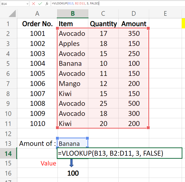
Let us take another example using the VLOOKUP function to find the results in different columns. Here we are trying to pick the Quantity and Amount of a specific item from the table and insert it in the Result column. 

Become a skilled Microsoft Excel professional with Microsoft Excel Masterclass - Sign up now! 

Example 2.1 

Let us take another example using the VLOOKUP function to find the results in different columns. Here we are trying to pick the Quantity and Amount of a specific item from the table and insert it in the Result column. Here's how you can do it:

STEP 1: First, select a cell where you want your value to be published.  

Start typing =VLOOKUP in your selected cell 
 

 

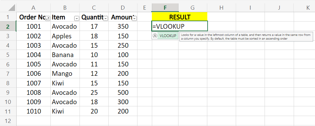
STEP 2:

Typing =VLOOKUP( will open a suggestion box to guide you in using the formula. 
 

 

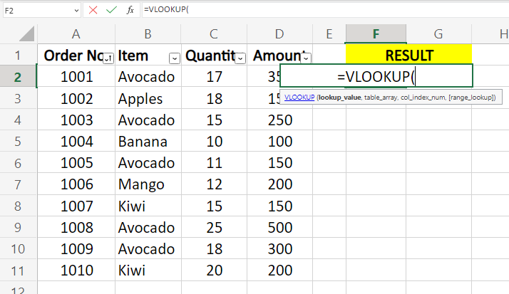
STEP 3:

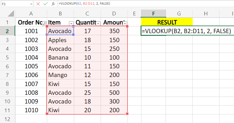
Then we will select a lookup value, that is Avocado in this case, in cell B2.  

Next, we will enter (,) or (;) and select the table array or the range where we want to find the lookup value and return value. It is (B2:D11) in this case. 
 

 

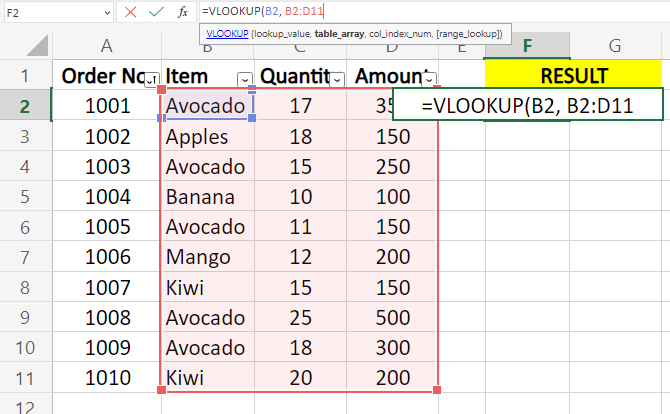
STEP 4:

We will enter (,) or (;) and the column number in which we want to look for the return value within the defined range. In the image below, we have entered 2, followed by the (,) and FALSE, to find the exact match. 
 

 

STEP 5:

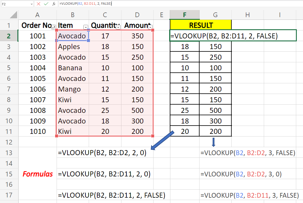
In this example 2.5, you can find the other values entered in the Result columns. To apply the formula to a particular range of cells below - enter a formula in a specific cell, and then you can click and drag from the bottom-right of the formulated cell to the cells below. 

In this case, the result for the applied formula in cell number F2 is 17. You can try the other formulas mentioned below in the image and find out what variations you can find in the Result column and range selection.
 

STEP 6:

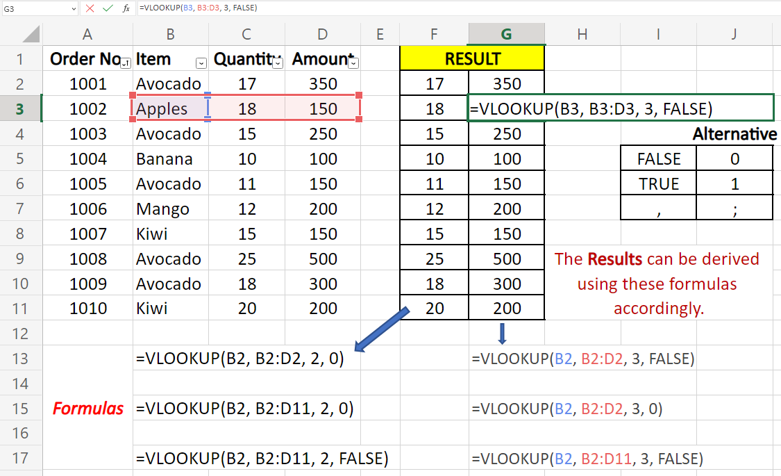
By trying these formulas, you will understand how you can change the lookup range and how it will affect the other cells when you drag and drop the applied instructions to the other cells. 
 

 

STEP 7:

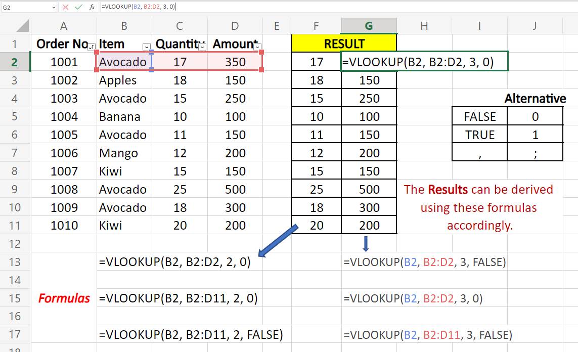
Irrespective of using FALSE or 0 in the formula (in result columns), the values derived in the result column remain the same. When using the VLOOKUP formula mentioned in cell G2 the lookup range is active for the cells B2, B2:D2 as highlighted in the image.  

As the applied VLOOKUP formula in the from the cell G2 is dragged and dropped in the cells below - the lookup range will change to ‘B3, B3:D3’, ‘B4, B4:D4’, and so on. 
 

 

You can try repeating our example once and then customise your formulas by setting the lookup value and table array (range) to find the lookup value and return value.  

Are you interested in upgrading your Excel skills? Join Microsoft Excel VBA and Macro Training course now! 

Example 3.1: Below we have given a third example showing - how you can sum up values from two tables for the same items using the VLOOKUP function.  

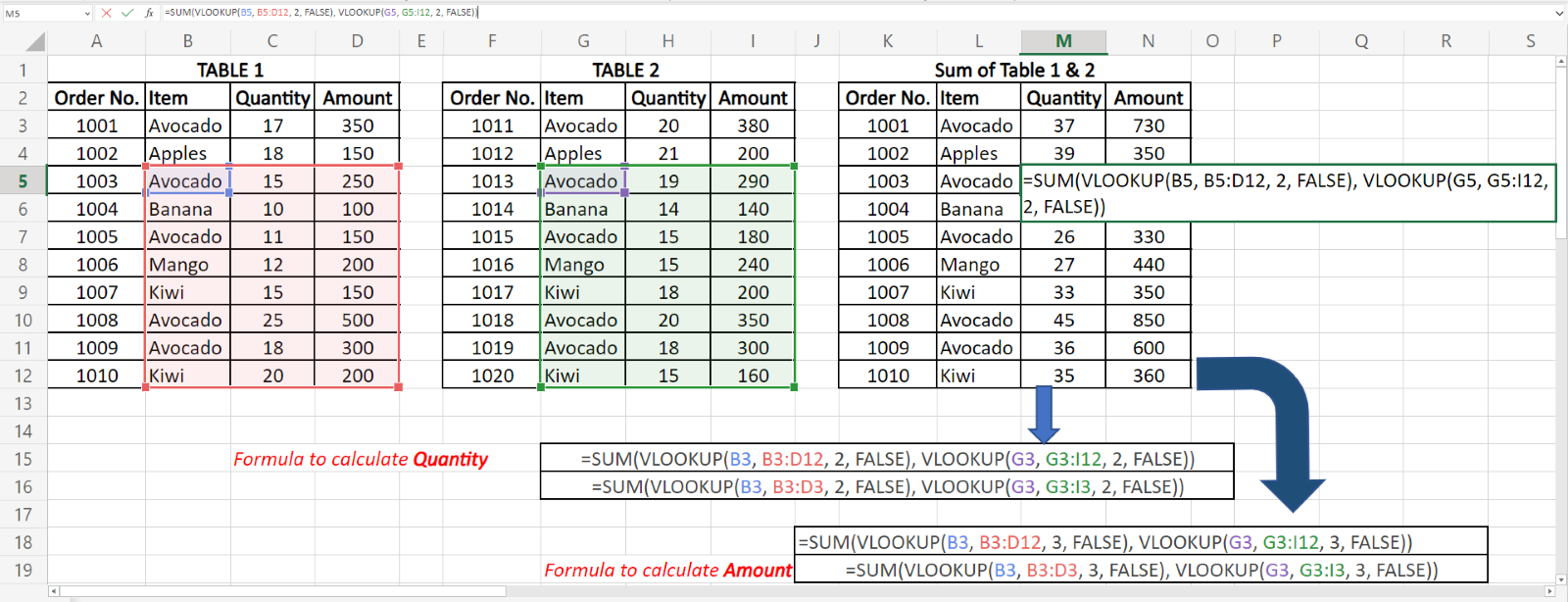
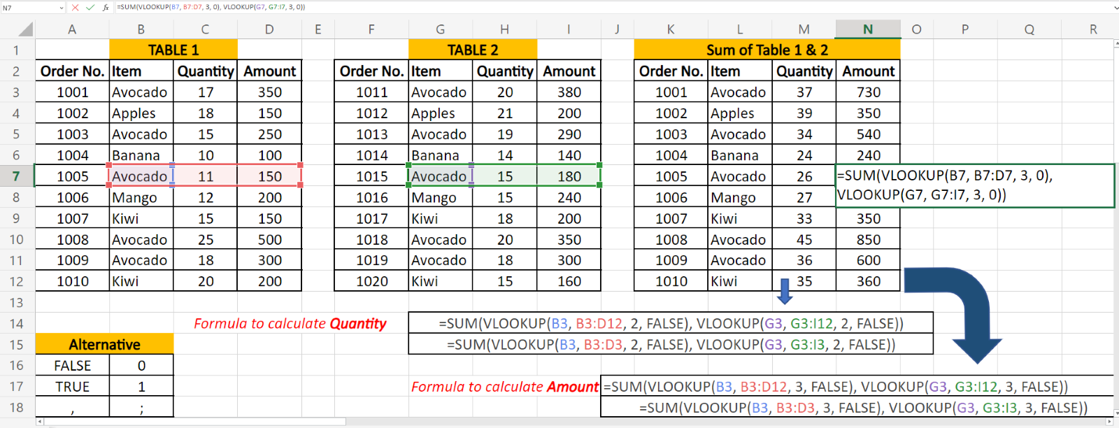
In the image below, we have two tables, table 1 and table 2, with the same items but different quantities and amounts for the specific order number. The third table in the image shows the sum of table 1 and table 2. It shows how the SUM function is used to add values in two different tables and bring them together at one table by integrating the SUM function and VLOOKUP formulas.   

Column number M5 in image 2.8 shows the formula used to calculate (sum) Quantity from table1 and table2. 
 

 

Example 3.2: Column number N7 in image 2.9 shows the formula used to calculate (sum) Quantity from table 1 and table 2. You can observe that ‘FALSE’ is replaced with ‘0’ in this formula, but the result remains unchanged. 
 

 

 

How to find an exact match using VLOOKUP? 

Finding an exact match for a value within the table is extremely easy. The steps to find an exact match using VLOOKUP are as follows:  

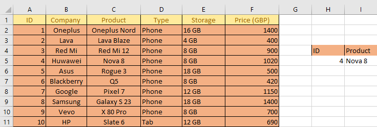
1) You can use the VLOOKUP function, as shown in the example below. This will allow you to find an exact match of the ID from the table. To do this, you must set parameters as a lookup value within a cell. In this case, the cell is H5. 
 

2) Next, you’ll need to specify the table’s location in the second argument. In this case, the table location would be A2:F11, as shown in the image.   

3) You need to specify the Column Index number next, which will let you know what value will be returned. The row you are looking up will return this value.  

4) Finally, you need to use a Boolean value, setting the value as FALSE. This will allow the VLOOKUP function to give you an exact match case for your value. If an exact value is not found, a N/A error will be displayed.
 

How to find approximate match using VLOOKUP?

An Approximate Match is a search case where you are returned the largest value after the lookup value, making it the closest value. Let's say you don’t have a present value within our table; Hence you can utilise the approximate Match function to find the solution.

To use an approximate match, you need to sort your first column in Ascending order. This would mean the data within your table would be arranged from A to Z based upon letters, and for numerical data, it will be sorted from least to the greatest numerical. The steps to perform an Approximate Match case are as follows: 

1) For the first step, we will copy a value from within a table and specify our lookup value. In this case, let's say the lookup value is 1020 GBP.
 

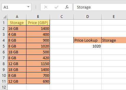
2) For the next step, you’ll need to determine a range for the relevant data and use the filter option to sort the values in the first column in ascending order. Once you have clicked on the filter options, the filter button is enabled within a column. Filter the data in ascending order and then click OK.
 

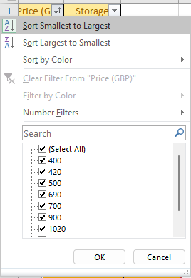
3) Use the VLOOKUP formula in the syntax and order mentioned before - the lookup value, table range, column number, and Boolean value. Set the value True for the Boolean argument, allowing you to find an approximate value. Once you’ve entered the LOOKUP formulae, press enter.
 

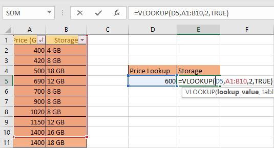
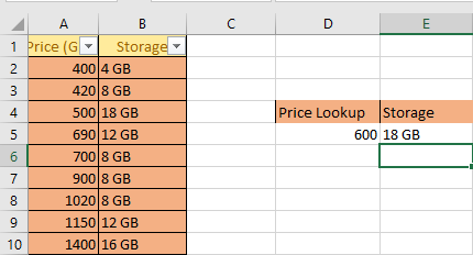
Example: Here, the return value is 18 GB of storage for 600 GBP.
 

Tips to use VLOOKUP Function Efficiently

It's common to encounter an error while working with the VLOOKUP function. If this generally happens to you, it might be because you are entering a formula incorrectly, or the value you entered might be wrong. Here is some general advice to use the VLOOKUP function more efficiently. 

1) Omitting the range_lookup from the LOOKUP function allows you to assess the non-exact match. But you should remember if it exists within your data, it will use an exact match. 

2) Only the first value will be picked if duplicate values are detected within the lookup column.  You can also find and remove duplicates in excel before using VLOOKUP.

3) You don’t need to worry about capitalising values, as VLOOKUP is not a case-sensitive function. 

4) VLOOKUP formulae will show an error if you add a column after applying the function. This results in an error because index values are hard coded, thus unable to change when a new column is added, or an old one is removed.

Conclusion

In this blog, we have seen a step-by-step process of using the VLOOKUP in Excel its formula with literal examples using this VLOOKUP function. To have a clear insight into the VLOOKUP function, you can practice with a few samples until you get familiar with it.

Learn how to create advanced formulas, macros and much more in our MS Excel training to become a Microsoft Excel Expert MO201 Training – join today!